Understanding Maximum Likelihood Estimation
Let’s say you collect some data from some distribution. As you might know, each distribution is just a function with some inputs. If you change the value of these inputs, the outputs will change (which you can clearly see if you plot the distribution with various sets of inputs).
It so happens that the data you collected were outputs from a distribution with a specific set of inputs. The goal of Maximum Likelihood Estimation (MLE) is to estimate which input values produced your data. It’s a bit like reverse engineering where your data came from.
In reality, you don’t actually sample data to estimate the parameter but rather solve for it theoretically; each parameter of the distribution will have its own function which will be the estimated value for the parameter.
How it’s done
First, assume the distribution of your data. For example, if you’re watching YouTube and tracking which videos have a clickbaity title and which don’t, you might assume a Binomial distribution.
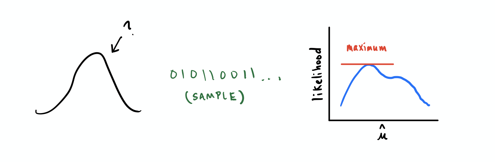
Next, “sample” data from this distribution whose inputs you still don’t know. Remember, you’re solving this theoretically so don’t need to actually get data as the values of your sample data won’t matter in the following derivation.
Now ask, what is the likelihood of getting the sample you got? Well, the likelihood would be the probability of getting your sample. And assuming each sample is independent from each other, we can define the likelihood function as:
$$ \begin{aligned} L(\theta_0, \theta_1, …; \text{sample 1}, \text{sample 2}, …) &= \P(X_1 = \text{sample 1}, X_2 = \text{sample 2}, …) \\\ &= \product{}{} \pmf(X_i) \end{aligned} $$
Now that you have your likelihood function, you want to find the value of the distribution’s parameter that maximizes the likelihood. It might help to think about the problem like this:
If you’re familiar with calculus, finding the maximum of a function involves differentiating it and setting it equal to zero. And if you actually differentiate the log of the function, it’ll make differentiation easier and you’ll get the same maximum.
Once you differentiate the log likelihood, just solve for the parameter. If you’re looking at the Bernoulli, Binomial, or Poisson distributions, you’ll only have one parameter to solve for. A Gaussian distribution will have two, etc…
Modeling YouTube views
Say you started a YouTube channel about a year ago. You’ve done quite well so far and have collected some data. You want to know the probability of at least $x$ visitors to your channel given some time period. The obvious choice in distributions is the Poisson distribution which depends only on one parameter, $\lambda$, which is the average number of occurrences per interval. We want to estimate this parameter using Maximum Likelihood Estimation.
We start with the likelihood function for the Poisson distribution:
$$ L(\lambda; x_1, …, x_n) = \product{i=1}{n} \frac{e^{-\lambda} \lambda^{x_i}}{x_i!} $$
Now take its log:
$$ \begin{aligned} \ln\bigg(\product{i=1}{n} \frac{e^{-\lambda} \lambda^{x_i}}{x_i!}\bigg) &= \summation{i=1}{n} \ln\bigg(\frac{e^{-\lambda} \lambda^{x_i}}{x_i!}\bigg) \\\ &= \summation{i=1}{n} [\ln(e^{- \lambda}) - \ln(x_i!) + \ln(\lambda^{x_i})] \\\ &= \summation{i=1}{n} [- \lambda - \ln(x_i!) + x_i \ln(\lambda)] \\\ &= -n\lambda - \summation{i=1}{n} \ln(x_i!) + \ln(\lambda) \summation{i=1}{n} x_i \end{aligned} $$
Then differentiate it and set the whole thing equal to zero:
$$ \begin{aligned} \frac{d}{d\lambda} \bigg(-n\lambda - \summation{i=1}{n} \ln(x_i!) + \ln(\lambda) \summation{i=1}{n} x_i \bigg) &= 0 \\\ -n + \frac{1}{\lambda} \summation{i=1}{n} x_i &= 0 \\\ \lambda &= \frac{1}{n} \summation{i=1}{n} x_i \end{aligned} $$
Now that you have a function for $\lambda$, just plug in your data and you’ll get an actual value. You can then use this value of $\lambda$ as input to the Poisson distribution to model your viewership over an interval of time. Cool, huh?
Maximizing the positive is the same as minimizing the negative
Now mathematically, maximizing the log likelihood is the same as minimizing the negative log likelihood. We can show this with a derivation similar to the one above:
Take the negative log likelihood:
$$ \begin{aligned} -\ln\bigg(\product{i=1}{n} \frac{e^{-\lambda} \lambda^{x_i}}{x_i!}\bigg) &= - \summation{i=1}{n} \ln\bigg(\frac{e^{-\lambda} \lambda^{x_i}}{x_i!}\bigg) \\\ &= - \summation{i=1}{n} [\ln(e^{- \lambda}) - \ln(x_i!) + \ln(\lambda^{x_i})] \\\ &= - \summation{i=1}{n} [- \lambda - \ln(x_i!) + x_i \ln(\lambda)] \\\ &= n\lambda + \summation{i=1}{n} \ln(x_i!) - \ln(\lambda) \summation{i=1}{n} x_i \end{aligned} $$
Then differentiate it and set the whole thing equal to zero:
$$ \begin{aligned} \frac{d}{d\lambda} \bigg(n\lambda + \summation{i=1}{n} \ln(x_i!) - \ln(\lambda) \summation{i=1}{n} x_i \bigg) &= 0 \\\ n - \frac{1}{\lambda} \summation{i=1}{n} x_i &= 0 \\\ \lambda &= \frac{1}{n} \summation{i=1}{n} x_i \end{aligned} $$
Now whether you maximize the log likelihood or minimize the negative log likelihood is up to you. But generally you’ll find maximization of the log likelihood more common.
Conclusion
Now you know how to use Maximum Likelihood Estimation! To recap, you just need to:
- Find the log likelihood
- Differentiate it
- Set the result equal to zero
- Then solve for your parameter