Understanding the Perceptron
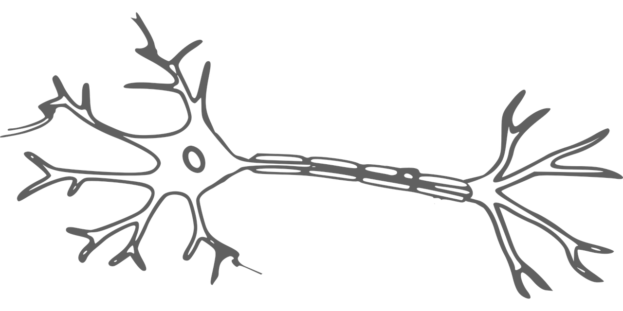
The perceptron model is a binary classifier whose classifications are based on a linear model. So, if your data is linearly separable, this model will find the hyperplane that separates it. The model works as such:
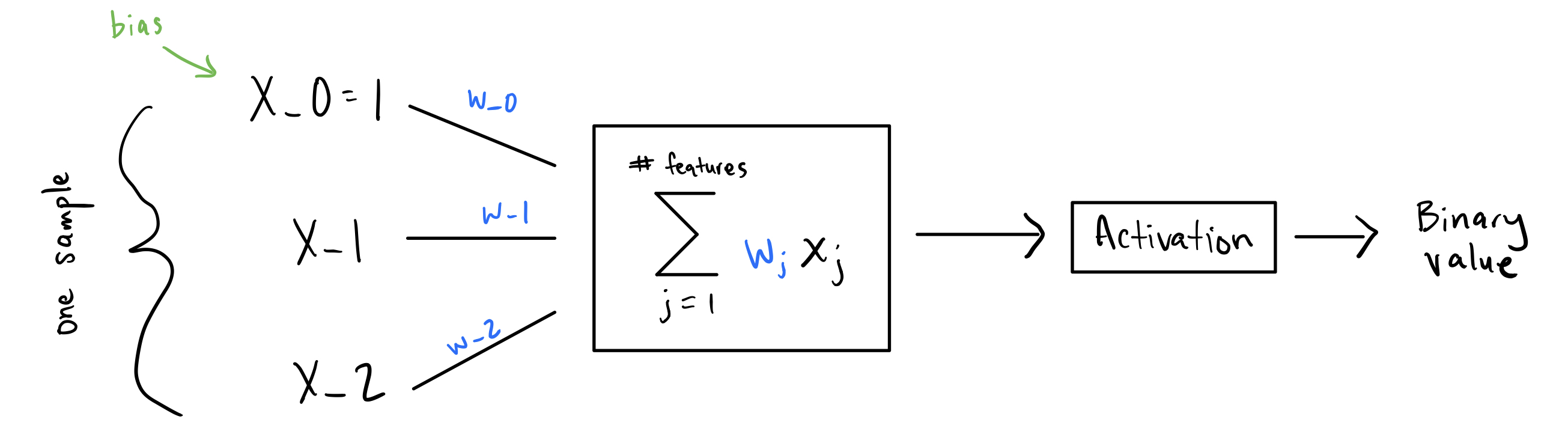
Essentially, for a given sample, you multiply each feature by its own weight and sum everything up - $\summation{j=1}{n} w_jx_j$. Then take this sum and apply the activation function. This will be your prediction. But which activation function do you use?
Activation functions
Binary classification labels generally appear as ${-1, 1}$ or ${0, 1}$. The activation function used in the perceptron model will depend on which set of binary labels you choose. If you choose ${0, 1}$, you will need to use the Heaviside step function as your activation function since it takes any real number and outputs either a 0 or a 1. Otherwise, you will use the sign function.
def sign(x):
    if x > 0:
        return 1.0
    elif x < 0:
        return -1.0
    else:
        return 0.0


def step(x):
    if x >= 0:
        return 1.0
    else:
        return 0.0
Get the data
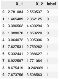
Say your binary labels are ${0, 1}$. The perceptron model prediction will be $\step\bigg(\summation{j=1}{n} w_jx_j\bigg)$, producing either a 0 or 1. Let’s look at a quick example with some data kindly pulled from Jason Brownlee’s blog Machine Learning Master.
import pandas as pd
import numpy as np

data = [[2.7810836,2.550537003,0],
        [1.465489372,2.362125076,0],
        [3.396561688,4.400293529,0],
        [1.38807019,1.850220317,0],
        [3.06407232,3.005305973,0],
        [7.627531214,2.759262235,1],
        [5.332441248,2.088626775,1],
        [6.922596716,1.77106367,1],
        [8.675418651,-0.242068655,1],
        [7.673756466,3.508563011,1]]

pd.DataFrame(data = data, index=list(range(len(data))), columns=['X_1', 'X_2', 'label'])
Let’s split the dataframe up into training data and labels.
train_data = pd.DataFrame(data = data, index=list(range(len(data))), columns=['X_1', 'X_2', 'label'])
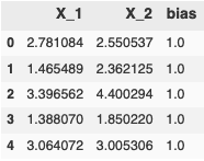
# Don't forget to add a vector of 1s for the bias weight
train_data['bias'] = np.repeat(1.0, train_data.shape[0])
train_label = train_data.label
train_data = train_data[[each for each in train_data.columns if each != 'label']]
train_data.head()
Perceptron inference
To get a prediction from the perceptron model, you need to implement $\step\bigg(\summation{j=1}{n} w_jx_j\bigg)$. Recall that the vectorized equivalent of $\step\bigg(\summation{j=1}{n} w_jx_j\bigg)$ is just $\step(w \cdot x)$, the dot product of the weights vector $w$ and the features vector $x$.
def activation(x, function_name):
    if function_name == 'step':
        return step(x)
    elif function_name == 'sign':
        return sign(x)
    else:
        raise NotImplementedError


def initialize_weights(num_columns):
    return np.zeros(num_columns)


def predict(vector, weights, activation_function):
    linear_sum = np.dot(weights, vector)
    output = activation(linear_sum, activation_function)
    return output
So you have $x$, which represents one sample where $x_i$ is some feature for the sample (like has_scales or has_fur if you’re trying to predict mammals vs. reptiles). But where do you get the weight $w_i$? This is what the perceptron model needs to learn from your labeled samples. At the start, you don’t know what these values should be, so you can just let them be all zeros.
Try predicting the first sample:
weights = initialize_weights(train_data.shape[1])
vector = train_data.loc[0].values
label = train_label.loc[0]
prediction = predict(vector, weights, 'step')
error = label - prediction
print(f'Prediction: {prediction}, Label: {label}, Error: {error}')
Prediction: 1.0, Label: 0, Error: -1.0
Unsurprisingly, the model doesn’t do such a great job. Let’s see if you can come up with a way for the perceptron model to learn what weights it needs to output the expected label.
Teaching the perceptron to learn
To begin, you need to specify a loss function which tells you how bad your model is doing. The lower the loss, the better. For our example, you can use the sum of squared errors as the loss function, $\summation{i=1}{m} (y_i - \yhat_i)^2$, where $\yhat_i$ is the perceptron model’s prediction and $y$ is what the prediction should have been (i.e. the label). This function simply determines the squared distance between the prediction and the true value and sums all these distances up.
As with most modern machine learning methods, you might be now be tempted to use gradient descent whereby you take the gradient of the loss function, $\summation{i=1}{m} (y_i - \yhat_i)^2$, with respect to the weights and use that gradient to update the weights in a direction that minimizes loss. The resulting gradient would be $-(y_i - \yhat_i) \frac{\partial \step(w \cdot x)}{\partial w_i} x_i$, but do you see the problem here? The derivative of the step function is 0 everywhere except at $x = 0$ where it’s undefined. This would force the entire gradient to be 0 and the weights would never be updated. The perceptron model would never learn. The same problem also plagues the sign function.
So how do you update the weights? Well, it turns out that if your data is linearly separable, then the following weight-update rule is guaranteed (via a convergence theorem proof) to converge to a set of weights in a finite number of steps that will linearly separate the data into two different classes. This update rule is defined as:
$$ w = w + y \cdot x $$
and only applied if $x$ was misclassified by the perceptron model.
But this update rule was derived under the assumption that the binary labels were ${-1, 1}$, not ${0, 1}$. If your labels were ${-1, 1}$, then $y$ in the update rule would be either -1 or 1, thus changing the direction in which the weights update.
But since your binary labels are ${0, 1}$, this presents a problem since $y$ could be 0. This would mean that if an $x$ got misclassified and its true value was 0, then $w = w + 0 \cdot x = w$ and the weights would never be updated.
Fortunately, you can account for this by amending the update rule that still guarantees convergence but is suited to both ${-1, 1}$ and ${0, 1}$ as the binary labels:
$$ w = w + (y - \yhat) \cdot x $$
Note that if your binary labels are ${0, 1}$, $(y - \yhat)$ is 0 if the perceptron model predicted correctly (thereby leaving the weights unchanged) and 1 or -1 if predicted incorrectly (which will ensure that the weights are updated in the right direction). If your binary labels are ${-1, 1}$, $(y - \yhat)$ is 0 if the perceptron model predicted correctly and 2 or -2 if predicted incorrectly. This amended weight-update rule ensures the correct directional change no matter which set of binary labels you choose.
Now that you know how to update the weights, try taking a sample, predicting its label, then updating the weights. Repeat this for each sample you have.
weights = initialize_weights(train_data.shape[1])
sum_of_squared_errors = 0.0
for sample in range(train_data.shape[0]):
    vector = train_data.loc[sample].values
    label = train_label.loc[sample]
    prediction = predict(vector, weights, 'step')
    error = label - prediction
    sum_of_squared_errors += error**2
    weights = weights + error * vector
print(f'SSE: {sum_of_squared_errors}')
print(f'Weights: {weights}')
SSE: 2.0
Weights: [4.84644761, 0.20872523, 0.]
Looks like the perceptron model didn’t find weights to perfectly separate the two classes yet. How about you give it more time to learn by taking multiple passes through the data. Let’s try 3 passes.
weights = initialize_weights(train_data.shape[1])
for epoch in range(3):
    sum_of_squared_errors = 0.0
    for sample in range(train_data.shape[0]):
        vector = train_data.loc[sample].values
        label = train_label.loc[sample]
        prediction = predict(vector, weights, 'step')
        error = label - prediction
        sum_of_squared_errors += error**2
        weights = weights + error * vector
    print(f'SSE: {sum_of_squared_errors}')
print(f'Weights: {weights}')
SSE: 2.0
SSE: 1.0
SSE: 0.0
Weights: [ 2.06536401, -2.34181177, -1.]
Nice! The sum of squared errors is zero which means the perceptron model doesn’t make any errors in separating the data.
Perceptron applied to different binary labels
Now say your binary labels are ${-1, 1}$. Using the same data above (replacing 0 with -1 for the label), you can apply the same perceptron algorithm. This time, you’ll see that $w = w + y \cdot x$ and $w = w + (y - \yhat) \cdot x$ both find a set of weights to separate the data correctly (even if the weights are different).
Here’s the perceptron model with $w = w + y \cdot x$ as the update rule:
weights = initialize_weights(train_data.shape[1])
for epoch in range(3):
    sum_of_squared_errors = 0.0
    for sample in range(train_data.shape[0]):
        vector = train_data.loc[sample].values
        label = train_label.loc[sample]
        if label == 0: label = -1
        prediction = predict(vector, weights, 'sign')
        error = label - prediction
        sum_of_squared_errors += error**2
        if error != 0:
            weights = weights + label * vector
    print(f'SSE: {sum_of_squared_errors}')
print(f'Weights: {weights}')
SSE: 5.0
SSE: 4.0
SSE: 0.0
Weights: [ 2.06536401, -2.34181177, -1.]
And now with $w = w + (y - \yhat) \cdot x$ as the update rule:
weights = initialize_weights(train_data.shape[1])
for epoch in range(3):
    sum_of_squared_errors = 0.0
    for sample in range(train_data.shape[0]):
        vector = train_data.loc[sample].values
        label = train_label.loc[sample]
        if label == 0: label = -1
        prediction = predict(vector, weights, 'sign')
        error = label - prediction
        sum_of_squared_errors += error**2
        weights = weights + error * vector
    print(f'SSE: {sum_of_squared_errors}')
print(f'Weights: {weights}')
SSE: 5.0
SSE: 8.0
SSE: 0.0
Weights: [ 3.98083288, -6.85733669, -3.]
Both converged!
Wrapping up
In the post, you’ve learned what a perceptron model is, what kind of data it can be applied to, the mathematics behind the model and how it learns, along with implementing all your findings in Python!
Of course in a realistic setting, you’ll want to cross-validate your model and preferably use a tried-and-true implementation of the model available in libraries like scikit-learn. But I hope this peak under the hood of the perceptron model has been helpful and if you have any questions, please feel free to reach out to me at bobbywlindsey.com or follow me on Medium or Twitter.