A Practical Look at Vectors and Your Data

I remember a feeling of utter confusion when I first learned vector spaces in my first course of Linear Algebra. What’s a space? And what are these vectors, really? Lists? Functions? Kittens? And how the hell does that relate to all this data that I analyze for some scientific endeavor? In this article, I attempt to explain the topic of vectors, vector spaces, and how they relate to data in a way that my former self would have appreciated.
The utility of the vector
Imagine a two-by-two graph as you might have seen in school. A vector is an object that’s typically seen in the form of an ordered list of elements, like (4, 3), that lives in a vector space and is commonly represented as an arrow whose tail starts at the origin, (0, 0), and ends at some other point, like (4, 3).
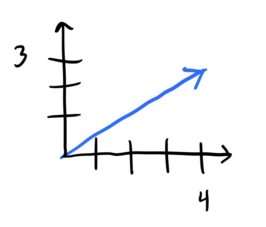
This arrow has a couple properties that are interesting to note: it has a direction and a length. A vector can represent many real-world objects like the wind, the throwing of a football, and the velocity of your car. It can even represent features of an animal, the quantities of your grocery list, or a row in your spreadsheet of data.
A space for your vectors
But how do you know if your object or ordered list is a vector? Well, it must belong to a set called a vector space. A vector space can be any set of elements (this could be lists, functions, or other objects) but these elements must follow some rules:
- Adding any two elements in the set results in another element that’s already in the set
- Multiplying any elements in the set by some number (called a scalar) results in another element that’s already in the set
- All the elements are associative, commutative, and scalars are distributive with respect to element addition
- There’s an element in the set such that adding it to any other element doesn’t change its value
- There’s some number (called a scalar) such that multiplying it by any other element doesn’t change the element’s value
- Any element in the set has some element that can be added to it which results in an element of 0s (called the zero vector)
If all the elements in your set follow the rules above, then congratulations! Your elements are called vectors and the set they belong to is called a vector space. But break any one of these rules, and you’re set is not a vector space and the elements inside your set aren’t vectors.
In mathematical jargon, these rules translate to the following:
- All elements are closed under addition
- All elements are closed under scalar multiplication
- All elements are associative, commutative, and scalars are distributive with respect to element addition
- An additive identity exists for every element
- A multiplicative identity exists for every element
- An additive inverse exists for every element
A tangible vector space
Consider the set you already know and love, $\R^2$. $\R^2$ is just $\R \cross \R$ which is the set of all possible two-dimensional lists represented by the following set notation ${(a, b) : a, b \in \R}$. You can visualize $\R^2$ below (obviously the x and y axes limits do not stop at ten but instead approach infinity):
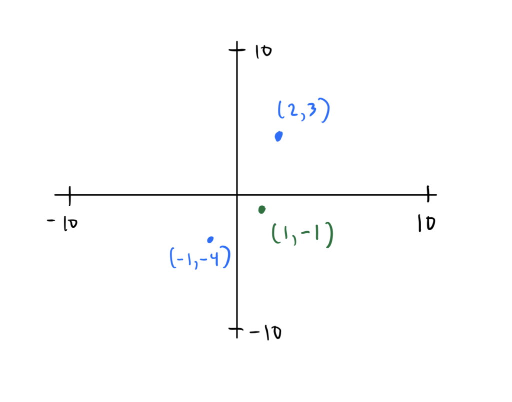
Is the set $\R^2$ a vector space? Well if it were, it would need to follow all the rules of a vector space that were mentioned above. Consider the first rule: adding any two elements in the set results in another element that’s already in the set. Does $\R^2$ follow this rule? Well, for example, take any two elements in $\R^2$, like (2, 3) and (-1, -4). When you add them together, do you get an element that’s also in $\R^2$? Yes! In fact, you get (1, -1) which does indeed live in the set $\R^2$. This is true for any two elements you add in $\R^2$ - you’ll always get something back that also belongs to $\R^2$.
So you’ve verified the first rule! But in order for $\R^2$ to be called a vector space, you must verify that it follows all the rules; which it does.
In short, there are many sets that follow the rules above so naturally you give it a name. And now when someone talks about some arbitrary set, you know that if the elements of the set follow the rules of a vector space, then the set must be a vector space.
Fields
Another note to make is about these scalars with which you can multiply vectors. Scalars are elements that belong to a set called a field which has the same rules as a vector space, but with the bonus of having a multiplicative inverse as well.
Since a field is a set that has all the rules a vector space has, then a field is also a vector space. You’ve actually been using fields all along, like the set of real numbers or the set of complex numbers. Any time you draw a plot on a two-dimensional grid, you’re actually drawing on a two-dimensional field.
Subspaces
In practice, you might think that it’s tedious to check every rule against a set to see if the set is a vector space. Well, you’re right. So that’s why it’s far easier to identify a set as a subset of a vector space you already know (like the set of real numbers) and prove that this subset is nonempty and that it’s closed under the same operations as the vector space (i.e. under addition and scalar multiplication).
If you’re able to do this, then your subset is called a subspace which also happens to be a vector space in and of itself (again, to see for yourself, take a subspace and verify that it has all the properties of a vector space).
So if you want to prove that a set is a vector space, try to prove that it’s a subspace instead. Since subspaces are vector spaces in their own right, you’ll have successfully shown that a set is a vector space.
Real-world data
Now all this theory is not very helpful if you can’t apply it. So consider the first few rows of the classic Iris dataset, which is a dataset containing samples of three different species of the Iris flower.
| Sepal Length | Sepal Width | Petal Length | Petal Width | Species |
|---|---|---|---|---|
| 5.1 | 3.5 | 1.4 | 0.2 | Iris-setosa |
| 4.9 | 3 | 1.4 | 0.2 | Iris-setosa |
| 7 | 3.2 | 4.7 | 1.4 | Iris-versicolor |
| 6.9 | 3.1 | 4.9 | 1.5 | Iris-versicolor |
| 6.3 | 3.3 | 6 | 2.5 | Iris-virginica |
| 7.1 | 3 | 5.9 | 2.1 | Iris-virginica |
As you can see from the header, the features of each sample are:
- sepal length
- sepal width
- petal length
- petal width
Each row of features can be viewed as an ordered list. The first list would be (5.1, 3.5, 1.4, 0.2), the second (4.9 , 3, 1.4, 0.2), and so on. But are these ordered lists vectors? Well, each entry in the lists is a real number and thus belongs to the set of real numbers, $\R$. And since each of these ordered lists are four-dimensional, then they live in $\R^4$. Since $\R^4$ is a vector space, then these ordered lists can be called vectors.
Notice that each entry in these vectors represents a dimension in $\R^4$ where each dimension corresponds to a feature in the dataset (like sepal length, sepal width, etc…). That is, each feature in your data can be considered a random variable. And since they’re random variables, we can do some descriptive statistics like find their means and standard deviations.
As you’ve already represented each row in the table as a vector, you can calculate the means and standard deviations of each random variable in one fell swoop. This is the power of vectors.
Pretend that the rows/vectors (5.1, 3.5, 1.4, 0.2) and (4.9 , 3, 1.4, 0.2) were all the data you had in the table above. Using two of the vector space rules, scalar multiplication and addition, we can easily calculate the means of every random variable we have.
$$ \frac{1}{2} \begin{bmatrix} 5.1 \\\ 3.5 \\\ 1.4 \\\ 0.2 \end{bmatrix}+ \frac{1}{2}\begin{bmatrix} 4.9 \\\ 3 \\\ 1.4 \\\ 0.2 \end{bmatrix}= \begin{bmatrix} 5 \\\ 3.25 \\\ 1.4 \\\ 0.2 \end{bmatrix} $$
So the mean of sepal length is 5, the mean of sepal width is 3.25, and so on. Representing your data as a set of vectors is not just aesthetically pleasing to look at, but also more performant in calculations since computers are optimized for computations involving vectors (turns out you can replace a lot of for loops with vector and matrix operations instead).
Conclusion
In the end, because you can represent your data as vectors which belong to a set with special rules called a vector space, many of the awesome things you do with your data like: linear feature transformations, standardizations, and dimensionality-reduction techniques can be justified by the rules of vector spaces.
And not only are vector spaces foundational to any work involving data, it constitutes the bedrock of linear algebra which is central to almost all areas of mathematics. Even if the phenomenon you’re studying is nonlinear, linear algebra is the go-to tool to use as a first-order approximation.
In short, vectors are tightly intertwined with your data and are very useful! So next time you’re importing data into a dataframe and performing a bunch of operations, remember that your computer is treating your data as a set of vectors and is happily applying transformations in a performant way. And all thanks to these little guys called vectors.