Understanding Linear Regression
Although linear regression models tend to be considered as a classical form of statistical modeling, it still remains to be widely deployed in many branches of science as a foundational tool to better understand data. A lot of online articles tend to either focus on just theory or take the other extreme of just writing a few lines of code to throw data at. As in most things in life, there’s a balance which I hope this post achieves.
Configure environment
from header import *
from sympy import *
init_printing(use_unicode=True)
import matplotlib.pyplot as plt
%matplotlib inline
plt.style.use('ggplot')
Get data
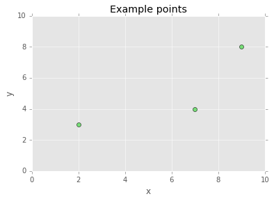
To understand a more complicated topic, it’s best to start with a simple problem whose insights can be scaled to much larger problems. In this spirit, let’s say you have a few data points: $(2, 3), (7, 4)$, and $(9, 8)$. We call each point and two-dimensional point since each point has two numbers. Using Python, you can easily generate and plot these points.
# put points in matrix
points = np.array([[2, 3], [7, 4], [9, 8]])

# plot styling
plt.title("Example points")
plt.xlabel("x")
plt.ylabel("y")
plt.xlim([0, 10])
plt.ylim([0, 10])

plt.plot(points[:, 0], points[:, 1], 'o', color="#77DD77")
Solving the system of equations
The goal is to model the trend in the data (to predict future unseen values) so we might want to draw a straight line that would hit all the points, but that’s not possible. Although you can easily see that a curved line would fit all the points, there’s actually a mathematical way you can prove that a straight line won’t cut it by using a system of equations. To create this system, use the equation for a straight line for each data point:
$$ \beta_0 + \beta_1x = y\ \mathrm{or}\ b + mx = y $$
and for each point you’ll get the following system of equations:
$\beta_0 + \beta_1 2 = 3$
$\beta_0 + \beta_1 7 = 4$
$\beta_0 + \beta_1 9 = 8$
Each $\beta_0$ is the coefficient for the intercept term (which is implicitly set to 1) so that by adjusting $\beta_0$, you can move the line up or down.
Since you might have much more data than the three points we have above, you’ll want to represent this system of equations in a way that is more computationally efficient for your computer to crunch. This can be achieved by using linear algebra notation:
$$ X \beta = y $$
which expands to…
$$ \left[\begin{matrix}1 & 2 \\ 1 & 7 \\ 1 & 9\end{matrix}\right] \left[\begin{matrix} \beta_1 \\ \beta_2\end{matrix}\right] = \left[\begin{matrix} 3 \\ 4 \\ 8 \end{matrix}\right] $$
We call $X$ the design matrix and $y$ the observation vector.
Now solve the system of equations! You can easily do this by using the row-reduced echelon (RRE) algorithm which is easily handled in Python.
# create design matrix
X = np.array([[1, 2], [1, 7], [1, 9]])
# observation vector
y = np.array([[3, 4, 8]])

augmented_matrix = Matrix(np.concatenate((X, y.T), axis=1))
printltx(r"Augmented Matrix =" + ltxmtx(augmented_matrix))

printltx(r"rref(Augemented Matrix) =" + ltxmtx(augmented_matrix.rref()[0]))
Augmented Matrix = $$\left[\begin{matrix}1.0 & 2.0 & 3.0 \\ 1.0 & 7.0 & 4.0 \\ 1.0 & 9.0 & 8.0\end{matrix}\right]$$
rref(Augemented Matrix) = $$\left[\begin{matrix}1.0 & 0 & 0 \\ 0 & 1.0 & 0 \\ 0 & 0 & 1.0\end{matrix}\right]$$
Look at the last row of rref(augmented matrix). This is saying that $0 = 1$ which is a contradiction! That’s the algorithm’s way of saying that the system of equations you made has no solution. In other words, you can’t find a fixed $\beta_0$ and $\beta_1$ that you could stick in the linear model you’re trying to build ($\beta_0 + \beta_1x = y$ which is just the equation for a line) that would satisfy all the x’s we have, $(2, 7, 9)$, and output all the $y$’s we have, $(3, 4, 8)$.
The below illustration shows that you can choose any $\beta_0$ and $\beta_1$, but it will always end up in the range of $X$ while never reaching $y = (3, 4, 8)$.
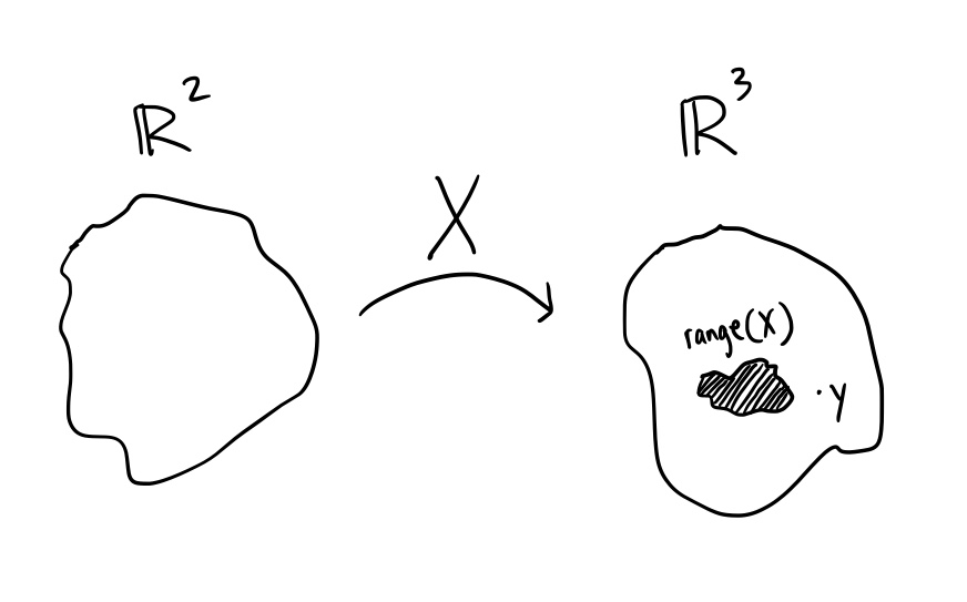
Estimate $\beta$ by projecting $y$ onto the range of $X$
Since $y$ is not in the range of $X$, the best you can do is come up with a close version of $y$ that is in the range of $X$. You can do this by “projecting” $y$ onto the range of $X$ (which will end up being some point in the range of $X$ that is closest to $y$).
There are two ways you can do this:
- the hard way
- orthogonalize your design matrix $X$ by using the Gram-Schmidt Algorithm
- the projection of $y$ onto the range of $X$ is $\hat{y} = \frac{\langle y, x_1 \rangle}{\langle x_1, x_1 \rangle}x_1 + \dots + \frac{\langle y, x_p \rangle}{\langle x_p, x_p \rangle}x_p$
- note that $\hat{y}$ is a target that can be hit
- and $\hat{y}$ is most like $y$
- solve $X \hat{\beta} = \hat{y}$
- the easy way
- use the solutions of the normal equation, $(X’X) \hat{\beta} = X’y$, which is the least squares solution to $X \beta = y$
- remember that $X \beta = y$ is what you were trying to solve earlier with the system of equations but couldn’t find a solution; the normal equation adjusts $y$ in the most minimal way as to give you an equation that will be solvable and leave you with $\hat{\beta}$s
- notice that $\hat{\beta}$s are not the same as $\beta$s since $\beta$s are the true parameters that we couldn’t find before using the system of equations and $\hat{\beta}$s are estimates of the true parameters
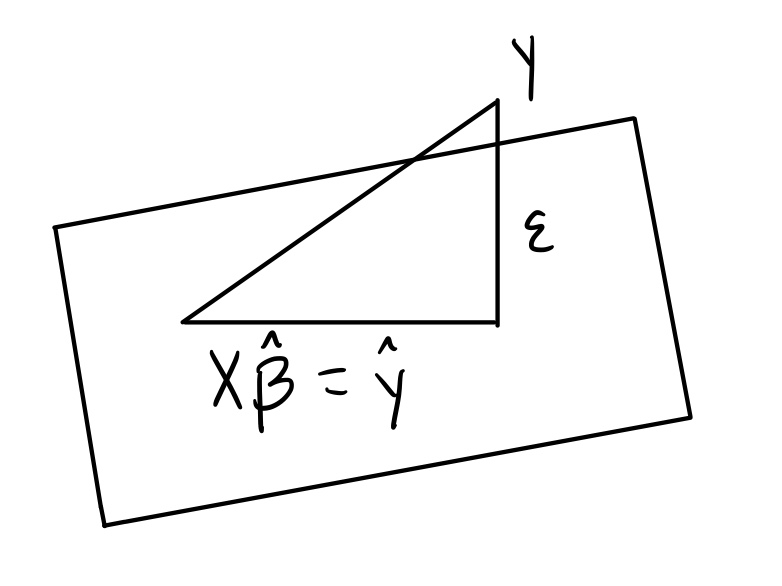
There’s a couple things to notice here:
- $\epsilon$, the residual vector, is perpendicular to $\hat{y}$ meaning that $\epsilon \perp \hat{y}$
- $\hat{y} + \epsilon = y$
One can also see the use of Pythagorean’s theorem at play here.
$\epsilon \perp \hat{y} \implies ||y||^2 = ||\hat{y} + \epsilon||^2 = ||\hat{y}||^2 + ||\epsilon||^2$
$\epsilon$ is minimized with $\hat{\beta}$
For this regression model, you want to show that the residual vector, $\epsilon$, is minimized with $\hat{\beta}$. To show that, you need to minimize the sum of squared errors which translates to minimizing $||y - X \beta||^2$. But to show $\beta$ is our best candidate, you need to start with an arbitrary candidate for our sum of squared errors, $|| y - X \gamma||^2$.
Firstly, you know that $y - X \gamma = y - X \hat{\beta} + X(\hat{\beta} - \gamma)$ because:
$$ \begin{aligned} y - X \gamma & = y - X \gamma + X \hat{\beta} - X \hat{\beta} \\ & = y - X \hat{\beta} + X \hat{\beta} - X \gamma \\ & = y - X \hat{\beta} + X(\hat{\beta} - \gamma) \\ \end{aligned} $$
Since you know $\epsilon \perp X$ by definition, then you can say that $|| y - X \gamma||^2 = ||y - X \hat{\beta}||^2 + ||X(\hat{\beta} - \gamma)||^2$.
Secondly, you use this fact to show that $||y - X \gamma||^2$ is minimized when $\gamma = \hat{\beta}$.
If $\gamma = \hat{\beta}$ then $||y - X \gamma||^2 = || y - X \hat{\beta}||^2$. And if $\gamma \ne \hat{\beta}$ then $||y - X \gamma||^2 = ||y - X \hat{\beta}||^2 + ||X(\hat{\beta} - \gamma)||^2$ which means $||y - X \hat{\beta}||^2 + ||X(\hat{\beta} - \gamma)||^2 \ge ||y - X \hat{\beta}||^2$.
So, $||y - X \gamma||^2$ is minimized when $\gamma = \hat{\beta}$.
Solving $X \hat{\beta} = \hat{y}$
Now we need to solve $X \hat{\beta} = \hat{y}$.
We know $\epsilon$ is orthogonal to every element in the range of $X$. So, we can say that $\epsilon \perp X \implies X \perp \epsilon \implies X’ \epsilon = 0$.
$X’ \epsilon = X’(y - X \hat{\beta}) = X’y - X’X \hat{\beta}$
So,
$$ \begin{aligned} X’y - X’X \hat{\beta} & = 0 \\\ X’X \hat{\beta} & = X’y\ \mathrm{(this\ is\ the\ normal\ equation)} \\\ \hat{\beta} & = (X’X)^{-1}X’y\ \mathrm{(the\ least\ squares\ solution)} \\\ \end{aligned} $$
Conclusion
Now that we know how to get our $\hat{\beta}$’s, we can use the design matrix, X, and our observation vector, y, to find the betas for our example. Plugging in X and y into $\hat{\beta} = (X’X)^{-1}X’y$, we get $\hat{\beta} = (1.30769231, 0.61538462)$ as shown in the Python code below (remember to transpose y to make it a column vector):
beta_hat = np.linalg.inv((X.T.dot(X))).dot(X.T).dot(y.T)
beta_hat
And there you have it! $\hat{\beta}$ is the vector containing each of the coefficients you were trying to find for your linear model and represents the closest thing we can get to a perfect solution.